How Linear Regression Works (With Python code)

By Md. Babul Hasan (NoYoN) 24 Jul, 2025 Post a Comment

How Linear Regression Works

A simple step-by-step guide with explanation + Python code

What is Linear Regression?

Linear Regression is a mathematical method for drawing the best straight line through a set of points. Imagine you're looking at different houses, and you notice something interesting:

Small houses cost less Big houses cost more

Now, you want to guess the price of a house just by knowing how big it is. So, you look at many houses and write down their size and price.

Then, you draw a straight line through all the dots on your paper. That line shows the pattern: as the house gets bigger, the price goes up.

That line is what we call a linear regression line helps us predict something — such as house prices — based on known information, like size.

Simple Example:

Imagine you know the sizes of some houses and how much they sold for. Now, if a friend asks,
“How much would a 1500 sq ft house cost?” → Linear regression helps you answer that question!

Step 1: The Equation of a Line

The core idea is to draw a line:

\hat{y} = \theta_0 + \theta_1 x

Where:

$x$ = input (e.g. house size)
$\hat{y}$ = predicted output (e.g. price)
$\theta_0$ = intercept (where the line crosses the y-axis)
$\theta_1$ = slope (how much price increases per unit of size)

This equation is referred to as our hypothesis or model.

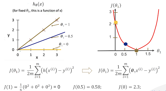
Step 2: Cost Function – How Good is Our Line?

To draw the “best” line, we need to know how far off our predictions are from real data.

We use something called a Cost Function (specifically, Mean Squared Error):

J(\theta_0, \theta_1) = \frac{1}{2m} \sum_{i=1}^m \left( h(x^{(i)}) - y^{(i)} \right)^2

This formula means:

Take the difference between the prediction and the actual result.
Square it so negatives don’t cancel out.
Add them all and take the average.

The smaller this value, the better our line.

Step 3: Gradient Descent – Making the Line Better

We now want to adjust θ₀ and θ₁ so the line gets better and better.

Gradient Descent is an algorithm that does exactly that:

\theta_j := \theta_j - \alpha \cdot \frac{\partial J}{\partial \theta_j}

Where:

$\alpha$ = learning rate (how fast to move)
$\frac{\partial J}{\partial \theta_j}$ = slope of cost (how to adjust)

Imagine you’re walking downhill — the goal is to reach the bottom (lowest error).

Step 4: Code Example in Python

Let’s code linear regression from scratch!

Goal: Predict house prices based on size

1. Import Libraries and Dataset

import numpy as np
import matplotlib.pyplot as plt

# Data: size (sq.ft) and price (lakh Taka)
X = np.array([280, 750, 1020, 1400, 1700, 2300, 2900])
Y = np.array([7.0, 22.4, 29.0, 40.9, 52.3, 70.5, 85.1])

2. Normalize Data

To make training smooth and fast, we scale everything between 0 and 1.

X_max = np.max(X)
Y_max = np.max(Y)

X = X / X_max
Y = Y / Y_max

3. Initialize Model

m = len(X)
X_train = np.ones((2, m))  # Add bias feature (x0 = 1)
X_train[1, :] = X
Y_train = Y.reshape(1, m)  # Make sure shape is (1, m)

def init_theta():
    return np.random.rand(1, 2)  # Random start for θ0, θ1

4. Define Key Functions

# Predict
def forward_prop(theta, X):
    return theta.dot(X)

# Cost Function
def compute_cost(h, Y):
    return (1 / (2 * m)) * np.sum((h - Y) ** 2)

# Gradient calculation
def backward_prop(h, Y, X):
    return (h - Y).dot(X.T)

# Update rule
def update_theta(theta, gradient, alpha):
    return theta - (alpha / m) * gradient

5. Train with Gradient Descent

def train(X, Y, alpha, iterations):
    theta = init_theta()
    for i in range(iterations):
        h = forward_prop(theta, X)
        gradient = backward_prop(h, Y, X)
        theta = update_theta(theta, gradient, alpha)

        if i % 100 == 0:
            cost = compute_cost(h, Y)
            print(f"Iteration {i} - Cost: {cost:.4f}")
    return theta

6. Predict New Prices

X_query = np.array([500, 1500, 2000]) / X_max

def predict(theta, X_vals):
    X_query = np.ones((2, X_vals.size))
    X_query[1, :] = X_vals
    return theta.dot(X_query)

# Train and predict
alpha = 0.1
iterations = 1000
theta = train(X_train, Y_train, alpha, iterations)

predicted = predict(theta, X_query) * Y_max
print("Predicted Prices:", predicted)

Sample Output:

Predicted Prices: [[14.27 44.53 59.66]]

That means:

500 sq.ft → approx. 14.27 lakh Taka
1500 sq.ft → approx. 44.53 lakh Taka
2000 sq.ft → approx. 59.66 lakh Taka

Visualize the Result

# Plot original data and the regression line
X_original = X * X_max
Y_original = Y * Y_max
pred_line = theta.dot(X_train) * Y_max

plt.scatter(X_original, Y_original, color='red', label="Training Data")
plt.plot(X_original, pred_line.flatten(), color='blue', label="Fitted Line")
plt.xlabel("Size (sq.ft)")
plt.ylabel("Price (Lakh Taka)")
plt.title("Linear Regression Example")
plt.legend()
plt.grid(True)
plt.show()

Programming & Tech Support

Widget HTML Atas